Portfolio rebalancing, Part 2: The private markets puzzle
Executive summary:
- Portfolios with large allocations to alternatives can have many benefits. However, alternatives allocations can deviate meaningfully from policy, particularly during periods of equity-market turbulence.
- One way to avoid this problem ahead of time is to be deliberate with assigning proxy asset classes.
- An overlay program can help manage a portfolio with an overweight to alternatives while also reducing unintended risk.
Editor’s note: This is the second in a three-part series on the topic of portfolio rebalancing.
Portfolios with large allocations to alternatives can reap benefits in many ways, with improved returns and diversification at the top of the list. However, some of those benefits are only possible due to their biggest drawback—illiquidity. The potential impact on the overall asset allocation from illiquidity can be meaningful, along with performance measurement distortions if not addressed.
At relatively small allocations of 5-10%, it’s difficult to stray too far from policy. But larger allocations of 30-50% can result in meaningful differences, particularly in volatile markets such as 2020 and 2022. This so-called denominator effect, resulting from the valuation lag on private assets, can quickly lead to a portfolio that’s 5-10% overweight to alternatives. We currently see this across a significant portion of our client base. In the absence of leverage, public assets will be meaningfully below targets—it’s just math. What are the best solutions in these cases?
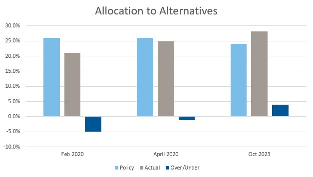
Exhibit 1 shows one such example. This client began February 2020 with a 5% underweight to alternatives. By April of that year, the sharp drop in liquid markets put them almost on policy. Now, in late 2023, while total assets have largely recovered, alternatives are now +4% overweight.
(Click image to enlarge)
Liquidating private assets can be very expensive, resulting in significant discounts to estimated values. Even stopping new commitments is often undesired as this can limit access to future investments when desired. In fact, our observations across client portfolios—and backed up with daily industry headlines—suggest that most investors are continuing to make new commitments. Given these dynamics, large overallocations are unlikely to reverse without a very strong bull market in liquid assets or making a deliberate change—either increasing the alternatives policy weight or stopping new commitments entirely.
How can an overallocation to alternatives be managed?
The most practical step is to be deliberate with assigning proxy asset classes. Given the mismatch in investment structures and valuation frequency, there is very little benefit to optimizations or returns-based analysis. I view this as more art than science—the best question to ask is “what liquid assets would I hold if I didn’t own alts?”
Private equity is arguably the easiest as public equity is typically viewed as a sensible substitute. Private credit and other fixed income related alternatives tend to group naturally with public fixed income. Other asset classes tend to have a broader range of classification. A common and practical approach for a diversified portfolio of alternatives is a hybrid proxy of equity and fixed income on a pro-rata basis. For example, an Absolute Return Strategy might be targeted as 50% equity and 50% fixed income. Or more practically, a pro-rata allocation across the current equity and fixed income policy weights. This is especially true when considering a broad allocation across multiple alternatives—if you didn’t own them, you would probably own proportionally more of the liquid assets.
What about performance measurement?
Many investors have their compensation linked to outperforming the policy benchmark representing a passive alternative. With so much riding on the outcome, it is critical to use the correct metrics. That is a very straightforward exercise in a portfolio of liquid public assets. Differences in asset class return versus benchmark are the result of selecting and assembling active managers with the intent of beating the benchmark. Unintended asset allocation differences are easily controlled, either through rebalancing physical assets or using a derivative overlay. The result is an easy determination of success or failure (I’ll leave the luck vs. skill question for others to debate).
The math changes greatly with alternatives. Benchmarks are, at best, imperfect representations of the asset class, often meaningless over the short term, and are not passively investible. Time horizons for measuring success or failure are necessarily longer. Even without any asset allocation deviations, performance deviations over the short term can be volatile. For example, private equity is typically benchmarked to public equity plus a premium, such as the Russell 3000 Index + 300 basis points (bps). In 2022, that benchmark was down -16%. Most private equity portfolios held their value, and many even appreciated. This 2,000+ basis points of alpha will dominate any measurement of success in the rest of the portfolio. Add to that an asset allocation effect of a 5-10% overweight and you see where this goes.
A better solution
To enhance performance measurement and attribution when investing in private assets, consider utilizing a second benchmark designed to eliminate the noise and focus on what is controllable. The policy portfolio is still the ultimate measuring stick, but adding a second “as invested” benchmark can be effective in the short term by recognizing what is controllable by the investor and what is simply noise.
For our derivative overlay clients, this is how we construct the adjusted policy targets which recognize the reality that the illiquid assets can’t be adjusted. This is essentially what any asset owner does in practice as well. Being overweight private equity doesn’t mean selling on the secondary market when it comes time to pay benefits. They sell liquid assets. Why not measure the decisions that are being made in the portfolio against a relevant benchmark?
Quantifying controllable vs. uncontrollable risk
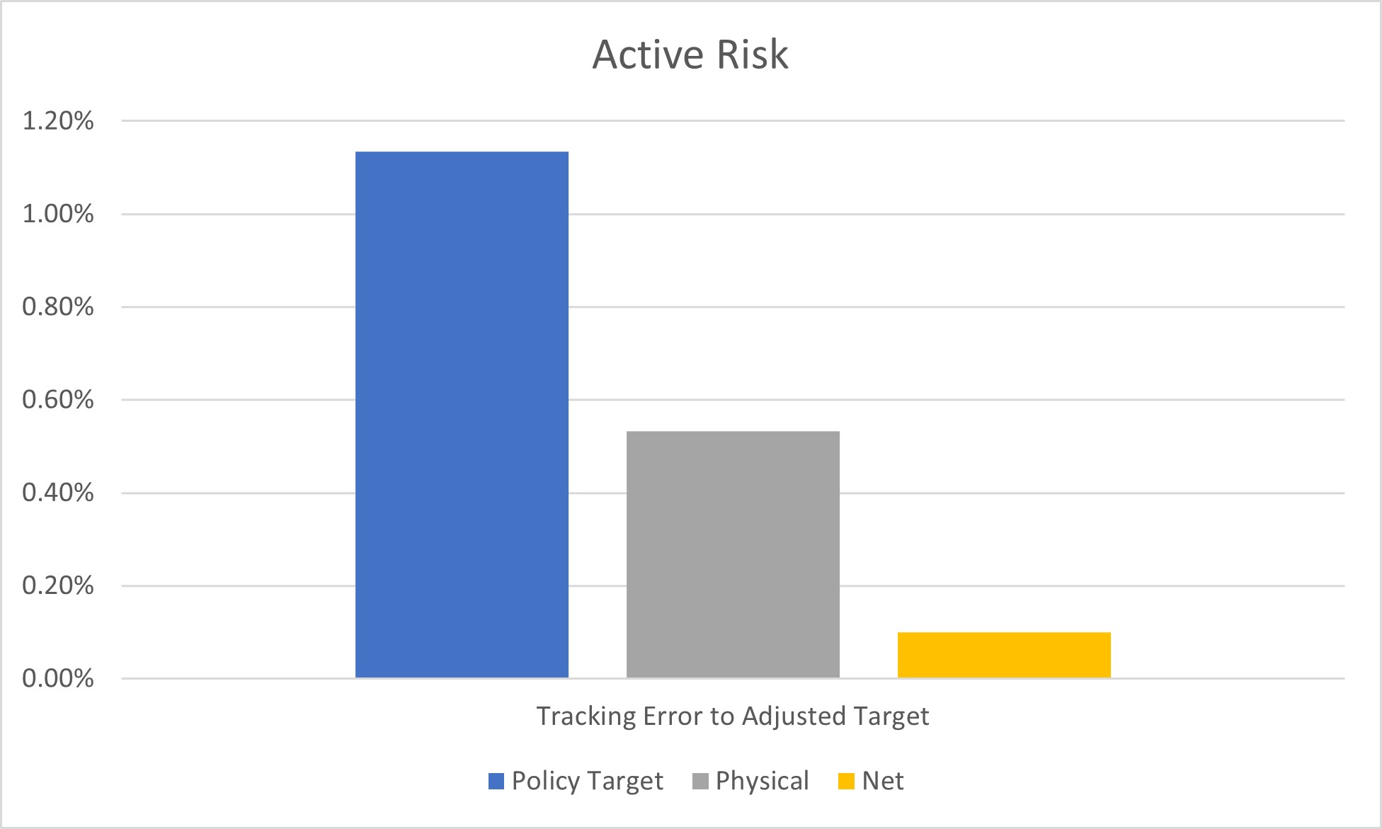
Let’s say that Client X has a 13% overweight to alternatives. How much of this risk is due purely to the exposure to alternatives and how much is controllable in liquid markets? We used our risk model to assess the ex-ante tracking error risk due to the difference in actual alternatives allocation to policy—uncontrollable risk—and then compared that to the adjusted policy, i.e., controllable risk. The results are shown in Exhibit 2 below.
Risk of Policy vs. Adjusted Policy = 113 bps
This risk is 100% due to the portfolio’s overweight position in alternatives and thus not controllable.
Risk of Physicals vs. Adjusted Policy = 53 bps
This risk is 100% due to cash held for liquidity purposes and mis-weights in liquid assets. Therefore, it is unintended, but controllable with very little cost.
(Click image to enlarge)
| Asset class | Policy | Physical | Adjusted Policy |
Physical + Overlay |
| Alternatives | 47.5% | 61.2% | 61.2% | 61.2% |
| Public Equity | 27.5% | 19.4% | 15.6% | 15.6% |
| Public Fixed Income | 25.0% | 17.7% | 23.2% | 23.2% |
| Cash | 0.0% | 1.7% | 0.0% | 0.0% |
| Total | 100.0% | 100.0% | 100.0% | 100.0% |
Risk of Net Exposure (Physical + Overlay) vs Adjusted Policy = 10 bps
Using an overlay to equitize cash held for liquidity and cash flows to rebalance the portfolio allows for seamless removal of 80% of the unintended risk, allowing active management decisions to flow through to the bottom line.
The case for overlays
While the risk model measures points in time, it lines up with our client experience, where we see typical risk reduction for the net exposures of 70-80% of tracking error to the adjusted policy. Ultimately, when it comes to managing unintended risk – and liquidity challenges – from an allocation to alternatives, we believe investors would be wise to consider adding a comprehensive overlay program.